Dataframe manipulation with dplyr

Table of Contents

• The dplyr package
• Using select()
• Using filter()
• Using group_by() and summarize()
• Using summarize()
• Using mutate()
• Challenge solutions
• Other great resources

Manipulation of dataframes means many things to many researchers, we often select certain observations (rows) or variables (columns), we often group the data by a certain variable(s), or we even calculate summary statistics. We can do these operations using the normal base R operations:

mean(titanic[titanic$Pclass == 1, "Age"],na.rm = TRUE)

[1] 38.23344

mean(titanic[titanic$Pclass == 2, "Age"],na.rm = TRUE)

[1] 29.87763

But this isn't very nice because there is a fair bit of repetition. Repeating yourself will cost you time, both now and later, and potentially introduce some nasty bugs.

The dplyr package

Luckily, the dplyr package provides a number of very useful functions for manipulating dataframes in a way that will reduce the above repetition, reduce the probability of making errors, and probably even save you some typing. As an added bonus, you might even find the dplyr grammar easier to read.

Here we're going to cover 6 of the most commonly used functions as well as using pipes (%>%) to combine them.

1. select()
2. filter()
3. group_by()
4. summarize()
5. mutate()

If you have have not installed this package earlier, please do so:

install.packages('dplyr')

Now let's load the package:

library(dplyr)

Using select()

If, for example, we wanted to move forward with only a few of the variables in our dataframe we could use the select() function. This will keep only the variables you select.

Name_Sex_Survived <- select(titanic,Name,Sex,Survived)

If we open up Name_Sex_Survived we'll see that it only contains the Name, Sex and Survived columns. Above we used 'normal' grammar, but the strengths of dplyr lie in combining several functions using pipes. Since the pipes grammar is unlike anything we've seen in R before, let's repeat what we've done above using pipes.

Name_Sex_Survived <- titanic %>% select(Name,Sex,Survived)

To help you understand why we wrote that in that way, let's walk through it step by step. First we summon the titanic dataframe and pass it on, using the pipe symbol %>%, to the next step, which is the select() function. In this case we don't specify which data object we use in the select() function since in gets that from the previous pipe.

Using filter()

If we now wanted to move forward with the above, but only with data for first class passengers, we can combine select and filter

Name_Sex_Survived_Female <- titanic %>%
    filter(Sex=="female") %>%
    select(Name,Sex,Survived)

As with last time, first we pass the titanic dataframe to the filter() function, then we pass the filtered version of the titanic dataframe to the select() function. Note: The order of operations is very important in this case. If we used 'select' first, filter would not be able to find the variable sex since we would have removed it in the previous step.

Using group_by() and summarize()

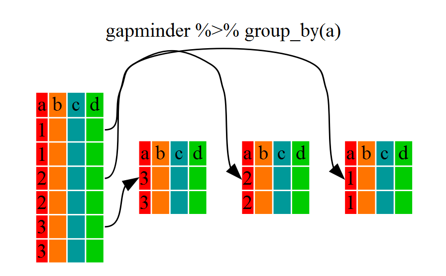
Now, we were supposed to be reducing the error prone repetitiveness of what can be done with base R, but up to now we haven't done that since we would have to repeat the above for each sex. Instead of filter(), which will only pass observations that meet your criteria (in the above: Sex=="female"), we can use group_by(), which will essentially use every unique criteria that you could have used in filter.

str(titanic)

'data.frame':    891 obs. of  12 variables:
 $ PassengerId: int  1 2 3 4 5 6 7 8 9 10 ...
 $ Survived   : int  0 1 1 1 0 0 0 0 1 1 ...
 $ Pclass     : int  3 1 3 1 3 3 1 3 3 2 ...
 $ Name       : Factor w/ 891 levels "Abbing, Mr. Anthony",..: 109 191 354 273 16 555 516 625 413 577 ...
 $ Sex        : Factor w/ 2 levels "female","male": 2 1 1 1 2 2 2 2 1 1 ...
 $ Age        : num  22 38 26 35 35 NA 54 2 27 14 ...
 $ SibSp      : int  1 1 0 1 0 0 0 3 0 1 ...
 $ Parch      : int  0 0 0 0 0 0 0 1 2 0 ...
 $ Ticket     : Factor w/ 681 levels "110152","110413",..: 524 597 670 50 473 276 86 396 345 133 ...
 $ Fare       : num  7.25 71.28 7.92 53.1 8.05 ...
 $ Cabin      : Factor w/ 148 levels "","A10","A14",..: 1 83 1 57 1 1 131 1 1 1 ...
 $ Embarked   : Factor w/ 4 levels "","C","Q","S": 4 2 4 4 4 3 4 4 4 2 ...

str(titanic %>% group_by(Sex))

Classes 'grouped_df', 'tbl_df', 'tbl' and 'data.frame':    891 obs. of  12 variables:
 $ PassengerId: int  1 2 3 4 5 6 7 8 9 10 ...
 $ Survived   : int  0 1 1 1 0 0 0 0 1 1 ...
 $ Pclass     : int  3 1 3 1 3 3 1 3 3 2 ...
 $ Name       : Factor w/ 891 levels "Abbing, Mr. Anthony",..: 109 191 354 273 16 555 516 625 413 577 ...
 $ Sex        : Factor w/ 2 levels "female","male": 2 1 1 1 2 2 2 2 1 1 ...
 $ Age        : num  22 38 26 35 35 NA 54 2 27 14 ...
 $ SibSp      : int  1 1 0 1 0 0 0 3 0 1 ...
 $ Parch      : int  0 0 0 0 0 0 0 1 2 0 ...
 $ Ticket     : Factor w/ 681 levels "110152","110413",..: 524 597 670 50 473 276 86 396 345 133 ...
 $ Fare       : num  7.25 71.28 7.92 53.1 8.05 ...
 $ Cabin      : Factor w/ 148 levels "","A10","A14",..: 1 83 1 57 1 1 131 1 1 1 ...
 $ Embarked   : Factor w/ 4 levels "","C","Q","S": 4 2 4 4 4 3 4 4 4 2 ...
 - attr(*, "vars")=List of 1
  ..$ : symbol Sex
 - attr(*, "drop")= logi TRUE
 - attr(*, "indices")=List of 2
  ..$ : int  1 2 3 8 9 10 11 14 15 18 ...
  ..$ : int  0 4 5 6 7 12 13 16 17 20 ...
 - attr(*, "group_sizes")= int  314 577
 - attr(*, "biggest_group_size")= int 577
 - attr(*, "labels")='data.frame':    2 obs. of  1 variable:
  ..$ Sex: Factor w/ 2 levels "female","male": 1 2
  ..- attr(*, "vars")=List of 1
  .. ..$ : symbol Sex
  ..- attr(*, "drop")= logi TRUE

You will notice that the structure of the dataframe where we used group_by() (grouped_df) is not the same as the original titanic (data.frame). A grouped_df can be thought of as a list where each item in the listis a data.frame which contains only the rows that correspond to the a particular value Sex (at least in the example above).

Using summarize()

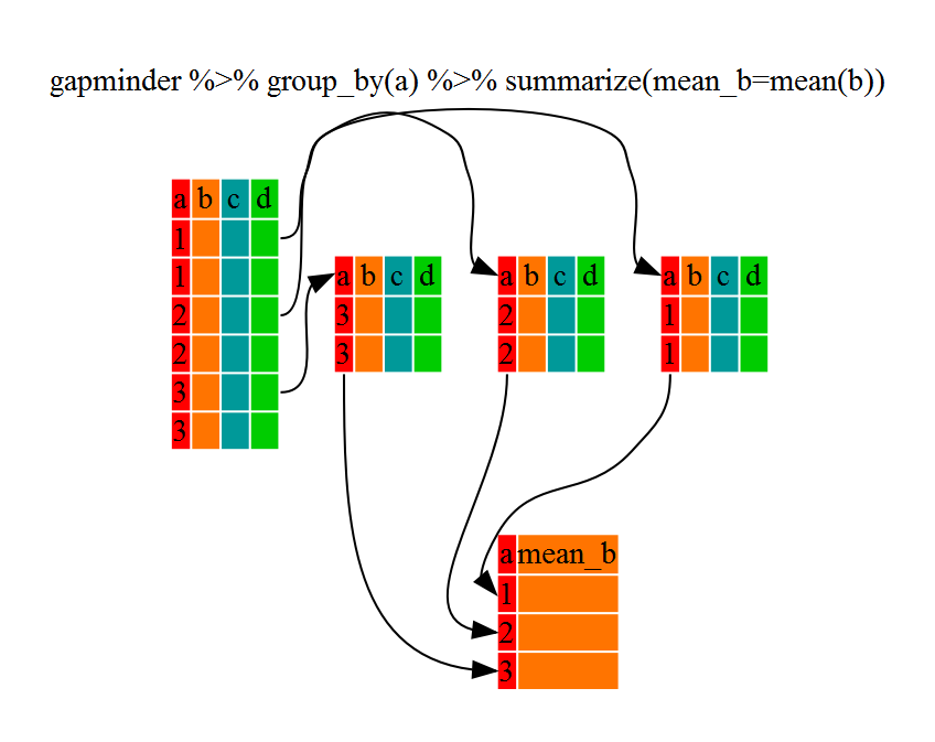
The above was a bit on the uneventful side because group_by() is only really useful in conjunction with summarize() (or summarise()). This will allow you to create new variable(s) by using functions that repeat for each of the sex-specific data frames. That is to say, using the group_by() function, we split our original dataframe into multiple pieces, then we can run functions (e.g. mean() or sd()) within summarize().

Survived_by_Sex <- titanic %>%
    group_by(Sex) %>%
    summarise(mean_Survived=mean(Survived))
Survived_by_Sex

Source: local data frame [2 x 2]

     Sex mean_Survived
  (fctr)         (dbl)
1 female     0.7420382
2   male     0.1889081

That allowed us to calculate the mean conscientiousness for each sex, but it gets even better. We can specify as many group_by variables as we want, enabling us to get stats on every combination of that set of variables.

That is already quite powerful, but it gets even better! You're not limited to defining 1 new variable in summarize().

Survived_by_PclassAndSex <- titanic %>%
    group_by(Pclass,Sex) %>%
    summarise(mean_Survived = mean(Survived),
              sd_Survived = sd(Survived),
              GroupSize = n())
Survived_by_PclassAndSex

Source: local data frame [6 x 5]
Groups: Pclass [?]

  Pclass    Sex mean_Survived sd_Survived GroupSize
   (int) (fctr)         (dbl)       (dbl)     (int)
1      1 female     0.9680851   0.1767160        94
2      1   male     0.3688525   0.4844835       122
3      2 female     0.9210526   0.2714484        76
4      2   male     0.1574074   0.3658823       108
5      3 female     0.5000000   0.5017452       144
6      3   male     0.1354467   0.3426942       347

Using mutate()

We can also create new variables prior to (or even after) summarizing information using mutate().

Survived_by_Sex_Status <- titanic %>%
    mutate(Status=Age*Pclass) %>%
    group_by(Sex) %>%
    summarize(mean_Age=mean(Age, na.rm = TRUE),
              sd_Age=sd(Age, na.rm = TRUE),
              mean_Status=mean(Status, na.rm = TRUE),
              sd_Status=sd(Status, na.rm = TRUE))
Survived_by_Sex_Status

Source: local data frame [2 x 5]

     Sex mean_Age   sd_Age mean_Status sd_Status
  (fctr)    (dbl)    (dbl)       (dbl)     (dbl)
1 female 27.91571 14.11015    53.05939  31.42541
2   male 30.72664 14.67820    67.05373  34.99498

Challenge solutions

Age_SibSp_Fare_Males <- titanic %>%
  filter(Sex=="male") %>%
  select(Age,SibSp,Fare)

Survived_by_PclassAndSex <- titanic %>%
    group_by(Pclass,Sex) %>%
    summarise(mean_Survived=mean(Survived))
Survived_by_PclassAndSex

Source: local data frame [6 x 3]
Groups: Pclass [?]

  Pclass    Sex mean_Survived
   (int) (fctr)         (dbl)
1      1 female     0.9680851
2      1   male     0.3688525
3      2 female     0.9210526
4      2   male     0.1574074
5      3 female     0.5000000
6      3   male     0.1354467

Survived_byPclass_RandomSample <- titanic %>% 
    filter(Sex=="female") %>%
    group_by(Pclass) %>%
    sample_n(20) %>%
    summarize(mean_Survived=mean(Survived)) %>%
    arrange(desc(Pclass))
Survived_byPclass_RandomSample

Source: local data frame [3 x 2]

  Pclass mean_Survived
   (int)         (dbl)
1      3          0.40
2      2          0.95
3      1          0.95

Other great resources

Data Wrangling Cheat sheet

Introduction to dplyr